The results presented on this site represent the current status of an ongoing project in the Solar Group at A&A of a reconstruction of the global structure of the solar wind in near-real-time using interplanetary scintillation (IPS) observations received daily from the Institute for Space-Earth Environmental Research (ISEE), Nagoya University, Japan. Our goal is to forecast solar wind conditions in the near-Earth environment, and predict the arrival of solar wind structures at Earth.
The reconstructions of the solar wind are based on a kinematic model of the solar wind. The density and velocity are specified on a source surface, typically located at 2.5 solar radii from the center of the Sun. Using this as a boundary condition, material is convected outward into the corona and heliosphere enforcing conservation of mass and mass flux where wind streams with different velocity interact.
An iterative least-squares algorithm is employed to obtain a 'best model' of the solar wind. Synthetic IPS velocity and IPS g-level data are calculated by integration through the solar wind model. Starting from an arbitrary initial state, differences between synthetic and actual IPS values are used to iteratively improve the model. Once the iterative procedure has converged, a solar wind model is obtained which provides the best possible fit with the IPS observations and is consistent with the kinematic model.
IPS observations are line-of-sight-integrated observations. The smearing inherent in these data, i.e., the ambiguity in determining where along a line of sight the observed signal originates, provides a serious challenge to any reconstruction. We use a tomographic technique to disentangle this line-of-sight smearing. Both solar rotation and outward motion of structures in the solar wind over time provide the views from different perspectives required for a tomographic analysis. See Jackson et al., 1998 for more details. The technique has been applied to IPS and Thomson scattering observations (examples).
We use observations from spacecraft instruments to provide corraborative space weather data. The SOHO/ LASCO coronagraphs observe solar wind structures (especially transient structures, such as CMEs) in the corona below 30 solar radii, before they can be detected by IPS radio systems; the Advanced Composition Explorer (ACE) spacecraft provides in situ velocity and density observations at the L1 Lagrange point, which can be compared with the values from our kinematic 'best model'.
![]()
Interplanetary scintillation (IPS) is caused by density fluctuations in the solar wind traveling across a line of sight extending from the observer out towards a compact radio source (e.g., a quasar), as illustrated in the figure on the left. Scattering and diffraction on these density fluctuations cause amplitude and phase changes in the incoming radio waves. The observed IPS signal is the result of contributions everywhere along the line of sight. The weight of each contribution depends on distance to the observer, observing frequency, source size and power spectrum of the fluctuations. The figure on the right shows this weight function for 327 MHz (the ISEE observing frequency), a source size of 1 arcsec and a spectrum power index of 3.
If the same radio source is observed simultaneously from multiple locations (typically three or four IPS stations are used), cross-correlation of the signals can be used to derive an IPS velocity, providing information about the solar wind velocity along the line of sight.
A single radio antenna will observe an IPS signal with a fluctuating power. These fluctuations, characterized as a scintillation index (or alternatively a g-level), provide information about the solar wind density along the line of sight to the IPS source.
Typically, IPS radio systems are operated as 'transit instruments': a selection of suitable IPS sources is observed once each day as the source transits across the local meridian at the observing site. These observations are analyzed to provide daily measurements of the IPS velocity and the scintillation index (or g-level).
This type measurement was pioneered by the IPS group at UCSD. As patterns of density fluctuations in the solar wind pass between Earth and a distant compact radio source incident radio waves are disturbed. This results in a pattern of intensity variations traveling across Earth's surface (somewhat similar to the shadows moving across the bottom of a swimming pool due to water ripples moving on the surface). If an IPS source is observed by several radio stations, then the IPS pattern moving across Earths' surface can be studied by cross-correlating the signals. In particular, the time lag of peaks in the cross-correlation function between stations determines the travel speed of the pattern (Coles and Kaufman, 1978). This measured speed is related to the solar wind speed everywhere along the line of sight towards the IPS source for a given day. In our tomographic model the IPS speed is described as a weighted mean of the solar wind speed along the line of sight.
These measurements have been pioneered by the IPS group in Cambridge (UK) (Hewish et al., 1964). Daily measurements of the scintillation strength of an IPS source over a prolonged period of time, plotted as a function of solar elongation (the angular distance in the sky of the source from the Sun), can be used to define a 'nominal' scintillation level to be expected from the IPS source when it is located at a given elongation under 'nominal' solar wind conditions. The figure on the right, from Gapper et al., 1982, illustrates this for a typical radio source. Crosses indicate daily observations; the solid line is the 'nominal' curve.
The g-level is defined as the ratio of the observed daily scintillation level and the 'nominal' value at the elongation of the IPS source. Days of high g-level (g>1) for a given source imply an increased level of small-scale scattering along the line of sight. A daily g-level measurement represents a weighted mean of the small-scale density fluctuations along the line of sight towards an IPS source for that day.
To help provide information about the solar wind density the small-scale density fluctuations in the solar wind need to be related to the density. This relationship is determined by empirically fitting g-level measurements to densities observed in situ near Earth (Tappin, S., 1986). Generally, high g-levels (i.e., high small-scale density fluctuations) imply larger solar wind densities along the line of sight to a given radio source.
 Currently, the IPS antenna system operated by the Solar-Terrestrial Environment
Laboratory (
ISEE)
of the Nagoya University in Japan is the only operational
system in the world that produces IPS velocity and g-level observations reliably
and continuously. Each year from spring to the beginning of winter (until weather
conditions force a shutdown) the ISEE IPS system observes about 20 IPS
sources close to the Sun each day, sampling the solar wind between 0.1 and 1.0 AU.
Currently, the IPS antenna system operated by the Solar-Terrestrial Environment
Laboratory (
ISEE)
of the Nagoya University in Japan is the only operational
system in the world that produces IPS velocity and g-level observations reliably
and continuously. Each year from spring to the beginning of winter (until weather
conditions force a shutdown) the ISEE IPS system observes about 20 IPS
sources close to the Sun each day, sampling the solar wind between 0.1 and 1.0 AU.
The ISEE system consists of antenna at four sites operating at an observing frequency of 327 MHz (wavelength of 0.92 m): Toyokawa, Fuji, Sugadaira and Kiso. IPS velocities are derived from observations at all four sites; g-level data are obtained from scintillation observations at Kiso only. The map on left shows the location of the four sites.
More information about the ISEE IPS antenna and IPS data is available on this ISEE web site. Some of the IPS observations are available here (this site also has 'life' pictures of the four IPS antennas).
ISEE runs its own forecast site, based on a tomographic technique similar to the one used at UCSD, using the same IPS data.
We show forecast results from two different models: a corotating (or time-independent) model and a time-dependent model.
The corotating model assumes that the solar wind structures observed by IPS do not change significantly over the time period used for the reconstruction, i.e., one solar rotation. Note that structures near the solar equator are essentially invisible to IPS while they are on the far side of the Sun, and are only observed over a substantial fraction of a solar rotation while they sweep past Earth from east to west. The reconstruction provides a single density and velocity distribution representing the average state of the solar wind during the rotation. This model is useful for studying slow changes (from one rotation to the next) in the structure of the solar wind. In addition, a comparison of this 'background' solar wind with the most recent IPS observations (as in the 'Sky Sweep' maps) provides a means of detecting transient heliospheric features. By averaging IPS data from a whole solar rotation to reconstruct a time-independent density and velocity distribution, the corotating model sacrifices time resolution for a better spatial resolution. For the ISEE data (with about 20 data points per day) the corotating model allows a reconstruction at a resolution of 10×10 degrees in heliographic latitude and longitude.
The time-dependent model allows for the evolution of solar wind structures over time scales much shorter than the solar rotation period. The purpose of this model is to track coronal mass ejections (CMEs) and other transient heliospheric features as they travel through the interplanetary medium, and forecast their arrival at Earth. This requires a time resolution on the order of one day (or better). Typically a time-dependent reconstruction covers about one solar rotation period in time steps of 1 day. The reconstruction provides a sequence of density and velocity distributions, each representing the average state of the solar wind over a 1-day period. For a 1-day time resolution the ISEE data allow a reconstruction with spatial resolution of 20×20 degrees in heliographic latitude and longitude.
Our reconstruction of the solar wind aims at deriving the density and the outflow velocity in the inner heliosphere where the data coverage by the IPS observations is sufficiently high to obtain reliable results.
Density and velocity are specified on an inner boundary (the source surface). The source surface is located at a heliocentric distance below all the IPS lines of sight, such that none of the lines of sight intersect the source surface. Typically a distance of 2.5 solar radii is used. Using density and velocity at the source surface as boundary condition the three-dimensional density and velocity follows using simple kinematic considerations and constraints on the solar wind outflow. We assume that solar wind outflow is strictly radial. Interactions between solar wind streams are dealt with by imposing conservation of mass and mass flux. Converging streams ('fast' solar wind catching up with 'slow' solar wind) merge, resulting in density and velocity consistent with the conservation rules.
The kinematic solar wind model determines the source location of material located anywhere in the heliosphere. Finding this source location is sometimes referred to as 'tracing back' to the source surface. The figure on the left illustrates this by 'tracing back' all locations along a line of sight to an IPS source. The blue line is the radial projection of the line of sight. The red line is the 'source location' of points along the line of sight assuming a constant solar wind speed of 400 km s-1 (note that the figure is not to scale: the source surface is actually located much closer to the Sun).
Due to the rotation of the Sun the source location is always located towards the west (larger heliographic longitude) of the radial projection on the source surface. Material observed at a location on the line of sight at a given time left the source location at an earlier time. In the case of a time-dependent model this 'source time' also needs to be taken into account.The reconstruction of the solar wind is based on an iterative least-squares algorithm. Starting from an arbitrary density and velocity distribution at the source surface, heliospheric distributions are calculated based on the kinematic solar wind model. Synthetic values for the IPS velocity and IPS g-level are obtained by integrating through the solar wind model. These are compared with the actual IPS observations. The differences between synthetic and actual IPS values provide the criterion to improve the model.
Each IPS line of sight is traced back to the source surface. This is illustrated for the corotating model in the figure on the right, showing the source surface as a Carrington map in heliographic coordinates. The dots divide the map into 10×10 degree bins. The positions of Earth on six subsequent days, traced back to the source surface, are shown as blue dots; for the same six days the traced-back positions of four lines of sight are shown in different colors. Where a sufficient number of projected lines of sight cross a given 10×10 degree bin on the source surface, contributions from all line-of-sight segments inside the bin, combined in a weighted mean, are used to improve the density and velocity values at the source surface. The weight for each segment is determined from the weight of the segment on the line of sight it belongs to (i.e., a point on the curve discussed in the section Interplanetary Scintillation), and the difference between synthetic and actual IPS data values. This update of the source surface completes one iteration.
Once the iteration process has converged a solar wind model is obtained that provides the best possible fit with the IPS observations, and is consistent with the kinematic solar wind model.
The quality of the reconstruction in each bin at the source surface improves as more lines of sight, after traceback to the source surface, cross the bin from many different directions. This requires that heliospheric structures that trace back to this bin are sampled by IPS from many different perspectives. This dependence on multiple perspectives is similar to classic tomography techniques as e.g. found in medicine; hence we call our technique 'heliospheric tomography'.
Changes in perspective result from two types of relative motion: corotation and solar wind outflow.
If observed structures do not change significantly over a solar rotation period, rotation past Earth (corotation; figure on left) provides views from widely different perspectives. The corotating model depends primarily on this first type of relative motion.
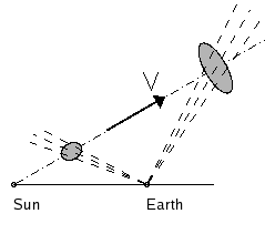
The time-dependent model requires that the viewing perspective changes on a time scale comparable to the time resolution, i.e., about one day. Corotation over this short period does not lead to a significant change in perspective. However, a large change in perspective does result from solar wind outflow (see figure to the right). This includes Earth-directed CMEs in addition to corotating structures.